MIT OCW - Introduction to Machine Learning - Week 1: Basics - Linear classifiers
Classification
A binary classifier is a mapping from $\mathbb{R}^d \rightarrow {-1, +1}$.
We’ll often use the letter $h$ (stands for hypothesis) to stand for a classifier, so the classification process looks like:
\[x \rightarrow h \rightarrow y\]But the value of $x$ is rarely a vector or a number. The $x$ we really want to classify is usually something like a song, an image, or a person.
In that case, we’ll have to define a function: $\varphi(x)$ with the domain is $\mathbb{R}^d$, where $\varphi$ represents features of $x$, like a person’s height or the amount of bass in a song.
Then, the entire function becomes:
\[h(\varphi(x)) \rightarrow \{-1, +1\}\]But the raw data is really noise, so we have to make one more step on filter out noise reflections on the data, then we use the function $\varphi(x)$ and we obtain number vectors.
So, the full process will be displayed below:
\[x \text{ (raw)} \rightarrow \varphi(x) \rightarrow \text{vector contains features of x (g)} \rightarrow h(g) \text{ can be -1 or +1}\]In supervised learning, we are given a training data set of the form
\[D_n = \{(x^{(1)}, y^{(1)}), \dots, (x^{(n)}, y^{(n)})\}\]We will assume that each $x^{(i)}$ is a $d \times 1$ column vector.
A classifier works well on new data is our target. To do that, we assume that there’s a connection between the training data and the testing data. Typically, they are drawn IID.
Given a training set and a particular classifier $h$, we can define the training error of $h$ to be:
\[\mathcal{E}_n(h) = \frac{1}{n} \sum_{i=1}^{n} \begin{cases} 1 & \text{if } h(x^{(i)}) \neq y^{(i)} \\ 0 & \text{otherwise} \end{cases}\]For now, we will try to find a classifier with small training error (later, with some added criteria) and hope it generalizes well to new data, and has a small test error
\[\mathcal{E}_n(h) = \frac{1}{n} \sum_{i=n+1}^{n+n'} \begin{cases} 1 & \text{if } h(x^{(i)}) \neq y^{(i)} \\ 0 & \text{otherwise} \end{cases}\]Learning algorithm
A hypothesis class $\mathcal{H}$ is a set (finite or infinite) of possible classifiers, each of which represents a mapping from $\mathbb{R}^d \rightarrow {-1, +1}$.
A learning algorithm is a procedure that takes a data set $\mathcal{D}_n$ as input and returns an element $h$ of $\mathcal{H}$, it looks like:
\[\mathcal{D}_n \longrightarrow \boxed{\text{learning alg}(\mathcal{H})} \longrightarrow h\]We will find that choice of $\mathcal{H}$ can have a big impact on the test error of the $h$ that results from this process. One way to get $h$ that generalizes well is to restrict the size, or expressiveness of $\mathcal{H}$.
Linear classifiers
We’ll start with the hypothesis class of linear classifiers. They are (relatively) easy to understand, simple in a mathematical sense, powerful on their own, and the basis for many other more sophisticated methods.
A linear classifier in $d-dimensions$ is defined by a vector of parameters $\theta \in \mathbb{R}^d$ and a scalar $\theta_0 \in \mathbb{R}$. So the hypothesis class $\mathcal{H}$ of linear classifiers is the set of all vectors in $\mathbb{R}^{d+1}$. We’ll assume that $\theta$ is an $d \times 1$ column vector.
Notes: Why is $R^{d+1}$ instead of $R^d$? It’s called parameter-bias merging (not an official term).
\[\tilde{x} = \begin{bmatrix} x \\ 1 \end{bmatrix} \in \mathbb{R}^{d+1}\] \[\tilde{\theta} = \begin{bmatrix} \theta \\ \theta_0 \end{bmatrix} \in \mathbb{R}^{d+1}\]Then, the linear classifier equation becomes:
\[h(x) = \tilde{\theta}^T \tilde{x}\]We can represent it with only a vector in $\mathbb{R^{d+1}}$.
Given particular values for $\theta$ and $\theta_0$, the classifier is defined by:
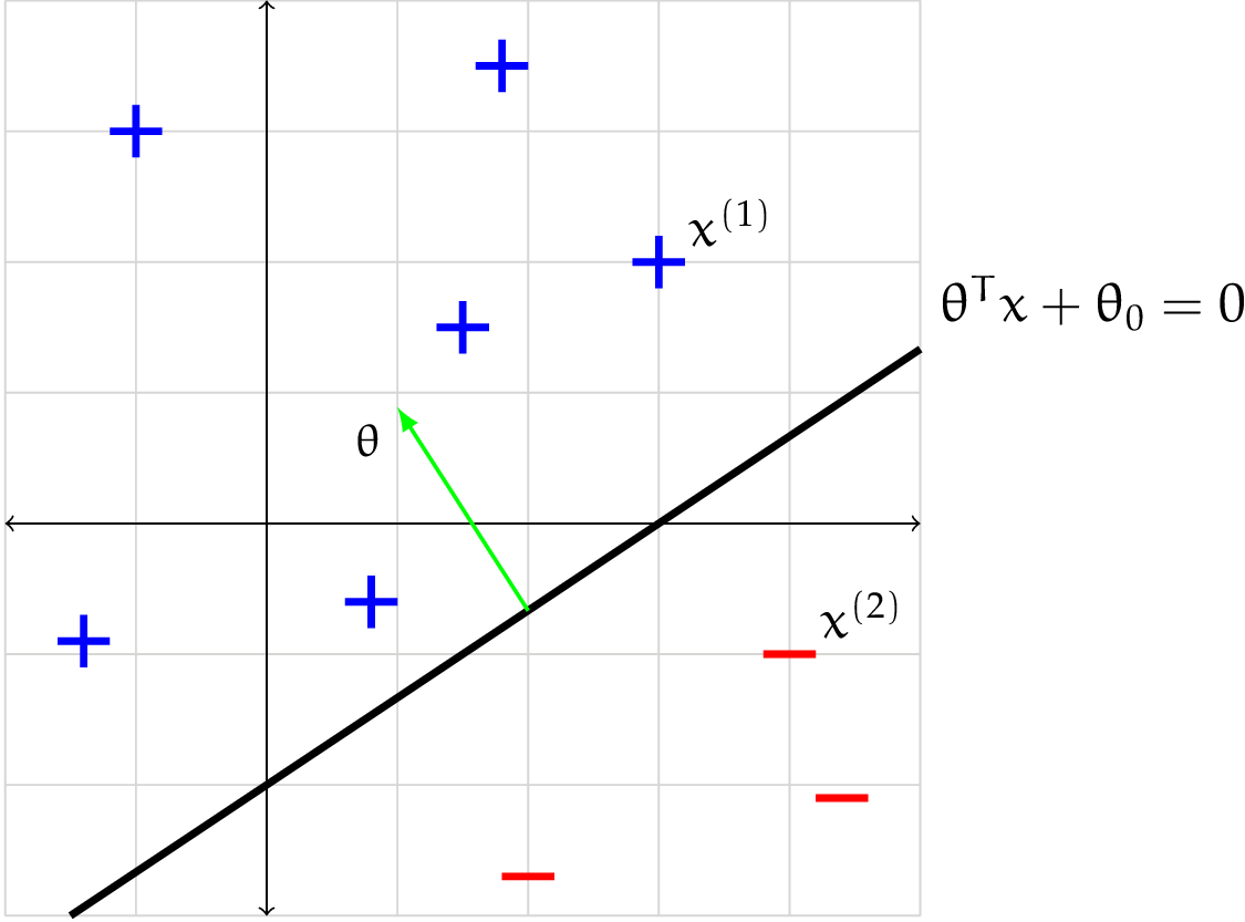
\[h(x; \theta, \theta_0) = \text{sign }(\theta^T x + \theta_0) \begin{cases} +1 & \text{if } (\theta^T x + \theta_0) > 0 \\ -1 & \text{ otherwise} \end{cases}\]It devides $\mathbb{R^d}$, the space that $x^{(i)}$ points live in, into 2 half-spaces. The one is on the same side as the normal vector is called the positive half-space, and we classify all points in that space as positive. Otehrwise, the other one is called negative half-space, and all points in that space is classified as negative.
Example: Let $h$ be the linear classifier defined by $\theta = \begin{bmatrix} -1 \ 1.5 \end{bmatrix}, \theta_0 = 3$.
In particular, let $x^{(1)} = \begin{bmatrix} 3 \ 2 \end{bmatrix}$ and $x^{(2)} = \begin{bmatrix} 4 \ -1 \end{bmatrix}$.
\[h(\mathbf{x}^{(1)}; \theta, \theta_0) = \text{sign}\left(\begin{bmatrix} -1 & 1.5 \end{bmatrix} \begin{bmatrix} 3 \\ 2 \end{bmatrix} + 3\right) = \text{sign}(3) = +1\] \[h(\mathbf{x}^{(2)}; \theta, \theta_0) = \text{sign}\left(\begin{bmatrix} -1 & 1.5 \end{bmatrix} \begin{bmatrix} 4 \\ -1 \end{bmatrix} + 3\right) = \text{sign}(-2.5) = -1\]Thus, $x^{(1)}$ and $x^{(2)}$ are given positive and negative classfications, respectively.
Learning linear classifiers
Now, given a data set and the hypothesis class of linear classifiers, our objective will be to find the linear classifier with the smallest possible training error.
Starting with a very simple learning algorithm. The idea is to generate $k$ possible hypotheses randomly. Then, we can evaluate the training-set error on each of the hypothesisi and return the hypothesis that gives the lowest training-set error.
Pseudo code:
1
2
3
4
5
6
7
8
Random-linear-classifiers(D, k, d)
{
    for j = 1 to k:
        theta_j = random(Rd)
        theta_0_j = random(R)
    ans = min-of-j that makes Epsilon_n(theta_j, theta_0_j) //training-set-error
    return (theta_ans, theta_0_ans)
}
Evaluating a learning algorithm
The best method to evaluate the efficiency of a learning algorithm is by using the new dataset and calculating the test-error on it.
It is too tricky to evaluate the performance of a learning algorithm. There’re many potential sources of variability in the possible result of computing test error on a learned hypothesis $h$:
Which particular training examples occured in $\mathcal{D}_n$.
Which particular testing examples occurred in $\mathcal{D}_{n’}$.
Randomization occured in the learning algorithm.
Generally, we would like to execute the following process multiple times:
Train on a new training set.
Evaluate the result $h$ on a new testing set.
In reality, we can divide a big dataset into parts. For example, we have the dataset $\mathcal{D}_n$, we divide it into $\mathcal{D}_1, \mathcal{D}_2, \dots$. It’s called cross validation.