MIT OCW - Introduction to Machine Learning - Week 2: Perceptron
Algorithm
We have a training dataset $\mathcal{D}_n$ with $x \in \mathbb{R}^d$ and $y \in {-1, +1}$.
The perceptron algorithm trains a binary classifier $h(x, \theta, \theta_0)$ using the following algorithm to find $\theta$ and $\theta_0$ using $t$ iterative steps:
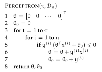
Looking at the algorithm’s pseudo code, we can see that on each step, if the current hypothesis defined with $\theta$ and $\theta_0$ classifies the example $x^{(i)}$ correctly, then no change is made, it’s all satisfied. Otherwise, the algorithm moves $\theta$ and $\theta_0$ so that it is closer to classifying $x^{(i)}, y^{(i)}$ correctly.
Note that if the algorithm ever goes through one iteration of the loop on line 4 without making an update, it will never make any further updates and so it should just terminate at that point.
Example: Let $h$ be the linear classifier defined by $\theta^{(0)} = \begin{bmatrix} 1 \ -1 \end{bmatrix}$ and $\theta_0^{(0)} = 1$. The diagram below shows several points classified by $h$. However, in this case, $h$ (represented by the bold line) misclassifies the point $x^{(1)} = \begin{bmatrix} 1 \ 3 \end{bmatrix}$, which has label $y^{(1)} = 1$.
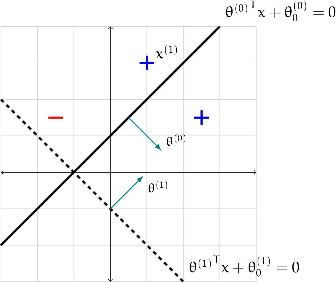
Running the Perceptron algorithm, we update:
\[\theta^{(1)} = \theta^{(0)} + y^{(1)}x^{(1)} = \begin{bmatrix} 2 \\ 2 \end{bmatrix}\] \[\theta_0^{(1)} = \theta_0^{(0)} + y^{(1)} = 2\]The new classifier (represented by the dashed line) now correctly classifies that point, but now makes a mistake on the negatively labeled point.
Offset
Sometimes, it can be easier to implement or analyze classifiers of the form
\[h(x; \theta) = \begin{cases} +1 & \text{ if } \theta^T x > 0 \\ -1 & \text{ otherwise} \end{cases}\]Without an explicit offset term $\theta_0$, this separator must pass through the origin, which may appear to be limiting.
However, we can convert any problem involving a linear separator with offset into one with no offset (but of higher dimension).
Consider the $d$-dimensional linear separator defined by $\theta = \begin{bmatrix} \theta_1 && \theta_2 && \dots && \theta_d \end{bmatrix}$ and offset $\theta_0$.
To each data point $x$ in dataset $\mathcal{D}$, append a coordinate with value $+1$:
\[x_{new} = \begin{bmatrix} x_1 && \dots && x_d && +1 \end{bmatrix}^T\]Define new $\theta$:
\[\theta_{new} = \begin{bmatrix} \theta_1 && \dots && \theta_d && \theta_0 \end{bmatrix}^T\]Then:
\[\theta_{new}^T \cdot x_{new} = \theta_1 x_1 + \dots + \theta_d x_d + \theta_0 \cdot 1\] \[= \theta^T x + \theta_0\]Thus, $\theta_new$ is an equivalent ($(d+1)$-dimensional separator to our original, but with no offset.
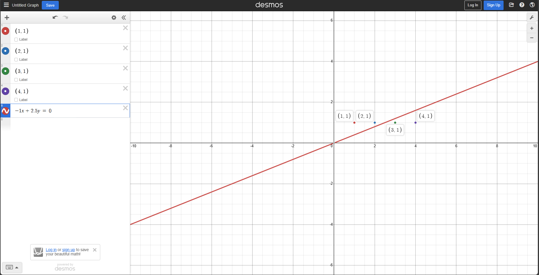
Consider the dataset:
\[X = [[1], [2], [3], [4]] Y = [[+1], [+1], [-1], [-1]]\]It is linearly separable in $d = 1$ with $\theta = [-1]$ and $\theta_0 = 2.5$. But it is not linearly separable through the origin. Now, let:
\[X_{\text{new}} = \begin{bmatrix} \begin{bmatrix} 1 \\ 1 \end{bmatrix} \begin{bmatrix} 2 \\ 1 \end{bmatrix} \begin{bmatrix} 3 \\ 1 \end{bmatrix} \begin{bmatrix} 4 \\ 1 \end{bmatrix} \end{bmatrix}\]This new dataset is separable through the origin, with $\theta_{new} = [-1, 2.5]^T$.
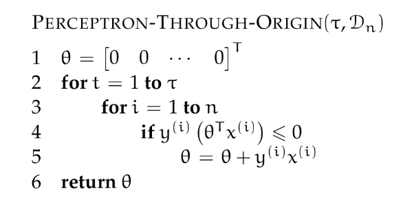
We can make a simplified version of the perceptron algorithm if we restrict ourselves to separators through the origin:
Theory of the Perceptron
Now, we’ll say something formal about how well the perceptron algorithm really works. We start by characterizing the set of problems that can be solved perfectly by the perceptron algorithm, and then prove that, in fact, it can solve these problems. In addition, we provide a notion of what makes a problem difficult for perceptron and link that notion of difficulty to the number of iterations the algorithm will take.
Linear separability
A training set $\mathcal{D}_n$ is linearly separable if there exist $\theta, \theta_0$ such that, for all $i = 1, 2, \dots, n$:
\[y^{(i)} (\theta^Tx^{(i)} + \theta_0) > 0\]Another way to say this is that all predictions on the training set are correct:
\[h(x^{(i)} ; \theta, \theta_0) = y^{(i)}\]And, another way to say this is that the training error is zero:
\[\mathcal{E}_n(h) = 0\]Convergence theorem
The basic result about the perceptron is that, if the training data $\mathcal{D}_n$ is linearly separable, then the perceptron algorithm is guaranteed to find a linear separator.
We will more specifically characterize the linear separability of the dataset by the margin of the separator. We’ll start by defining the margin of a point with respect to a hyperplane.
First, recall that the distance of a point $x$ to the hyperplane $\theta, \theta_0$ is:
\[\frac{\theta^Tx + \theta_0}{||\theta||}\]Then, we’ll define the margin of a labeled point $(x, y)$ with respect to hyperplane $\theta, \theta_0$ to be:
\[y \cdot \frac{\theta^Tx + \theta_0}{||\theta||}\]This quantity will be positive if and only if the point $x$ is classified as $y$ by the linear classifier by this hyperplane.
Study Question: What sign does the margin have if the point is incorrectly classified? Be sure you can explain why.
Answer: Based on the above formular, y will be $+1$ or $-1$. The perpendicular distance expressed by the rest. This value is signed, so if the sign of the result returned is different to $y$, the point is incorrectly classified, and the margin is negative.
Now, the margin of a dataset $\mathcal{D}_n$ with respect to the hyperplane $\theta, \theta_0$ is the minimum margin of any point with respect to $\theta, \theta_0$:
\[\min_i y^{(i)} \cdot \frac{\theta^T x^{(i)} + \theta_0}{||\theta||}\]The margin is positive if and only if all the points in the dataset are classified correctly. In that case, it represents the distance from the hyperplane to the closest point.
Exercises
1. Classification
Consider a linear classifier through the origin in 4 dimensions, specified by
\[\theta = (1, -1, 2, -3)\]Which of the following points $x$ are classified as positive, i.e. $h(x;\theta) = +1$?
$(1, -1, 2, -3)$
$(1, 2, 3, 4)$
$(-1, -1, -1, -1)$
$(1, 1, 1, 1)$
Solution: The vector $\theta \in R^4$ creates a hyperplane through the origin, which is $\theta^Tx$.
If $\theta^Tx$ > 0, it means the point $x$ is on the positive side of the hyperplane. Else, if the value is negative, it indicates that the point $x$ is on the negative side of the hyperplane. On the case that $\theta^Tx = 0$, the point is exactly on the hyperplane.
Now, we only need to calculate $\theta^Tx$ with the given points respectively.
1
2
3
4
5
6
7
8
9
10
11
12
13
14
15
import numpy as np

theta = np.array([1, -1, 2, -3])

points = [
    (1, -1, 2, -3),
    (1, 2, 3, 4),
    (-1, -1, -1, -1),
    (1, 1, 1, 1)
]

for x in points:
    x_array = np.array(x);
    result = np.dot(theta, x_array)
    print(result)
The value returned:
1
2
3
4
15
-7
1
-1
So, the answer will be [1, 3] in the form of Python list.
2. Classifier vs Hyperplane
Consider another parameter vector:
\[\theta' = (-1, 1, -2, 3)\]Ex2a: Does $\theta’$ represent the same hyperplane as $\theta$ does?
Yes, although $\theta$ and $\theta’$ have opposite signs, they define the same hyperplane (just as in $\mathbb{R}^2$ two lines coincide, in $\mathbb{R}^3$ to planes coincide).
Ex2b: Does $\theta’$ represent the same classifier as $\theta$ does?
No, although they have the same hyperplane, the classifier depends on the direction of the vector, since the two vectors have the opposite direction, they do not represent the same classifier.
3. Linearly Separable Training
$\mathcal{E}_n(\theta, \theta_0)$ refers to the training error of the linear classifier specified by $\theta, \theta_0$ and $\mathcal{E}(\theta, \theta_0)$ refers to its test error. What does the fact that the training data are linearly separable imply?
Select “yes” or “no” for each of the following statements:
Ex3a: There must exist $\theta, \theta_0$ such that $\mathcal{E}(\theta, \theta_0) = 0$.
No. Even if the training data is separable, test error can be non-zero, especially if the test data has noise or is from a slightly different distribution.
Ex3b: There must exist $\theta, \theta_0$ such that $\mathcal{E}_n(\theta, \theta_0) = 0$.
Yes. A linear classifier exists that perfectly separates the training data.
Ex3c: A separator with 0 training error exists
Same idea as above. Linearly separable means a separator with 0 training error does exist.
Ex3d: A separator with 0 testing error exists, for all possible test sets
No. We can’t guarantee 0 test error for all test sets. Overfitting or distributional shifts may cause test error > 0, even with perfect training accuracy.
Ex3e: The perceptron algorithm will find $\theta, \theta_0$ such that $\mathcal{E}_n(\theta, \theta_0) = 0$.
Yes. If the training data is linearly separable, the perceptron algorithm is guaranteed to converge to a solution with 0 training error.
4. Separable Through Origin?
Provide two points, $(x_0, x_1)$ and $(y_0, y_1)$ in two dimensions that are linearly separable but not linearly separable through the origin.
We can recognize that the two points satisfying the above condition lie in the same quadrant of the $Oxy$ coordinate system, and also lie in the same straight line passing through the origin. For example:
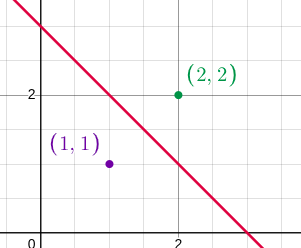
Two points: $(1, 1)$ and $(2, 2)$ and the label are $-1$ and $+1$ respectively. The red line’s equation is $x + y = 3$. There isn’t any line passing through the origin which classifies that 2 points correctly.
Week 2 Homework
1. Perceptron mistakes
Let’s apply the perceptron algorithm (through the origin) to a small training set containing three points:
\[x^{(1)} = [1, -1], y^{(1)} = 1 \\ x^{(2)} = [0, 1], y^{(2)} = -1 \\ x^{(3)} = [-1.5, -1], y^{(3)} = 1\]Given that the algorithm starts with $\theta{(0)} = [0, 0]$, the first point that the algorithm sees is always a mistake. The algorithm starts with some data points (to be specified in this question), and then cycles through the data until it makes no further mistakes.
1.1. Take 1
Initialize $\theta = [0, 0]$. The hyperplane will be a line coincides with $x$-axis. Check if the line classifying the points correctly. If it doesn’t, updating $\theta$ base on the Perceptron algorithm. The initialization case below:
Point’s label is $+1 \rightarrow$ mistake, updating $\theta$, starts with $x^{(1)}$:
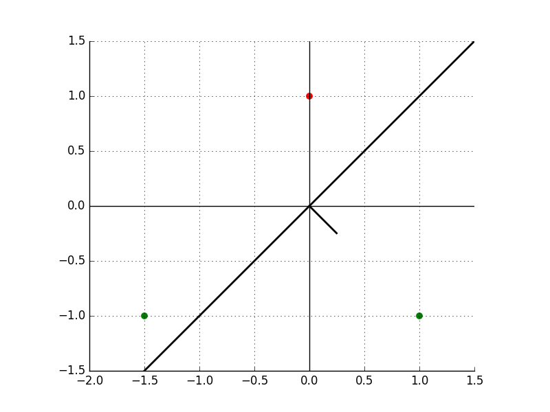
\[\theta = \theta + y^{(1)} x^{(1)} = [0, 0] + 1 \cdot [1, -1] = [1, -1]\]Corresponding to the line: $x - y = 0$ in 2-dimension, and the direction is downward.
Continue to $x^{(2)}$, prediction:
\[\theta^T \cdot x = [1, -1]^T \cdot [0, 1] = -1\]It is correct, no update.
Continue to $x^{(3)}$, prediction:
\[\theta^T \cdot x = [1, -1] \cdot [-1.5, -1] = -0.5\]while the label is $+1 \rightarrow$ need to update:
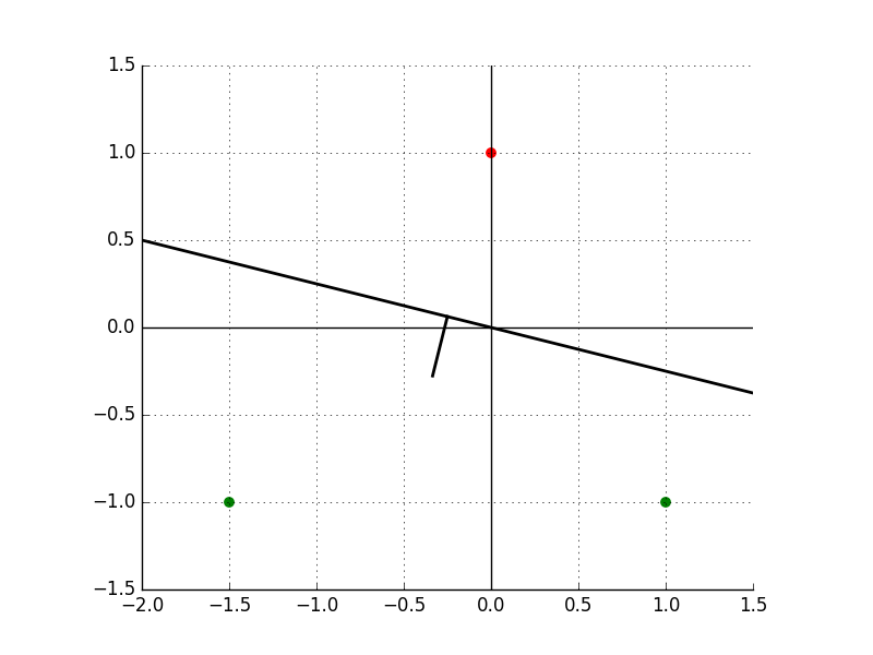
\[\theta = \theta + y^{(3)} x^{(3)} = [1, -1] + 1 \cdot [-1.5, -1] = [-0.5, -2]\]Corresponding to the line: $-0.5x - 2y = 0$, represented in the below graph:
Back to $x^{(1)}$, the prediction:
\[\theta^T \cdot x = [-0.5, -2] \cdot [1, -1] = 1.5\]It is correct, no update. Continue to $x^{(2)}$, the prediction:
\[\theta^T \cdot x = [-0.5, -2] \cdot [0, 1] = -2\]It is correct, no update. Continue to $x^{(3)}$, the prediction:
\[\theta^T \cdot x = [-0.5, -2] \cdot [-1.5, -1] = 2.75\]It is also correct, no more mistake.
1.1a: How many mistakes does the algorithm make until convergence if the algorithm starts with data point $x^{(1)}$?
The answer is 2.
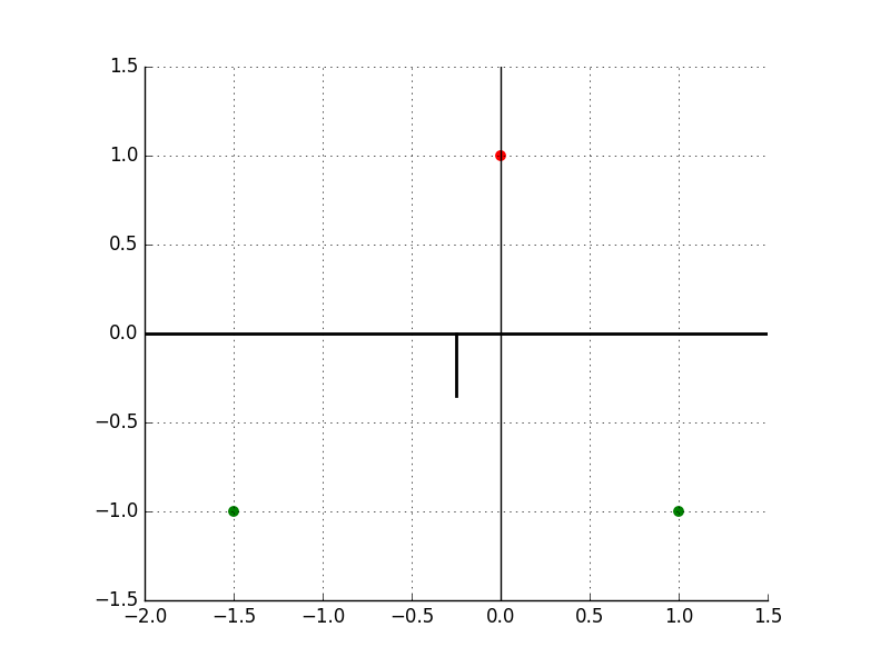
1.1b: Which of the above plot(s) correspond to the progression of the hyperplane as the algorithm cycles? Ignore the initial 0 weights, and include an entry only when $\theta$ changes.
Please provide the plot number(s) in the order of progression as a Python list.
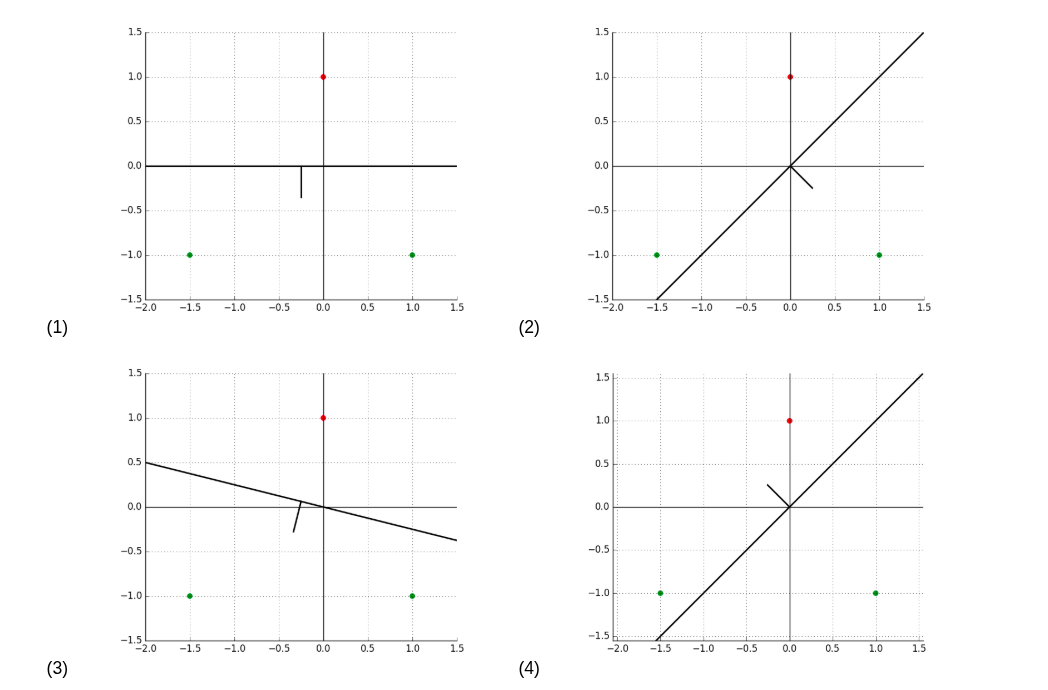
The given process. The answer is [2, 3]. Plot 2 shows the change after step 1 with $x^{(1)}$. Plot 3 shows the change after step 3 with $x^{(3)}$.
Both questions below is similar to the previous questions. Giving answer only.
1.1c: How many mistakes does the algorithm make if it starts with data point $x^{(2)}$, and then does $x^{(3)}$ and $x^{(1)}$.
The answer is 1, after step 1 with $x^{(2)}$.
1.1d: Again, if it starts with data point $x^{(2)}$, and then does $x^{(3)}$ and $x^{(1)}$, which plot(s) correspond to the progression of the hyperplane as the algorithm cycles? Ignore the initial 0 weights.
Please provide the plot number(s) in the order of progression as a Python list.
The answer is [1].
1.2. Take 2
This test is completely similar to Take 1.
2. Initialization
2.1. If we were to initialize the perceptron algorithm with $\theta = [1000, -1000]$, how would it affect the number of mistakes made in order to separate the data set from question 1?
Answer: It would significantly increase the number of mistakes.
Explaination: The Perceptron algorithm updates $\theta$ when it misclassifies a data point (make mistakes). The initial value of $\theta$ can greatly influence early predictions, and thus, the number of mistakes made.
With the data set given in question 1, the value of points are too small, when the initial value of $\theta$ is far larger. So, it “takes more time” to modify the value of $\theta$ in order to be closer to the points. Then, it would significantly increase the number of mistakes.
2.2. Provide a value of $\theta^{(0)}$ for which running the perceptron algorithm (through origin) on the data set from question 1 returns a different result than using $\theta^{(0)} = [0, 0]$.
Answer: $\theta = [1, 1]$.
Try $\theta = [1, 1]$:
First, $x_1 = [1, -1], y_1 = 1$:
\[\theta^T x_1 = 0 \text{ (wrong)} \rightarrow update: \theta = [1, 1] + [1, -1] = [2, 0]\]Next, testing on $x_2 = [0, 1], y_2 = -1$:
\[\theta^T x_2 = 0 \text{ (wrong)} \rightarrow update: \theta = [2, 0] - [0, 1] = [2, -1]\]Then, testing on $x_3 = [-1.5, -1], y_3 = 1$:
\[\theta^T x_3 = -2 \text{ (wrong)} \rightarrow update: \theta = [2, -1] + [-1.5, -1] = [0.5, -2]\]It’s different from $[-0.5, -2]$ when initial value of $\theta$ is $[0,0]$.