MIT OCW - Introduction to Machine Learning - Week 3: Features
Linear classifiers and the XOR dataset
Linear classifiers are easy to work with and analyze, but they are a very restricted class of hypotheses. If we have to make a complex distinction in low dimensions, then they are unhelpful.
Our favorite illustrative example is the “exclusive or” (xor) data set, the drosophila of machine-learning data sets:

There is no linear separator for this two-dimensional dataset! But, we have a trick available: take a low-dimensional data set and move it, using a non-linear transformation into a higher-dimensional space, and look for a linear separator there. Let’s look at an example data set that starts in 1-D:
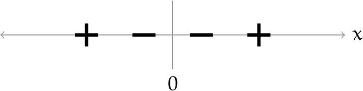
These points are not linearly separable (in 1D, a linear separator is a point), but consider the transformation $\phi(x) = [x, x^2]$. Putting the data in $\phi$ space, we see that it is now separable. There are lots of possible separators; we have just shown one of them here.
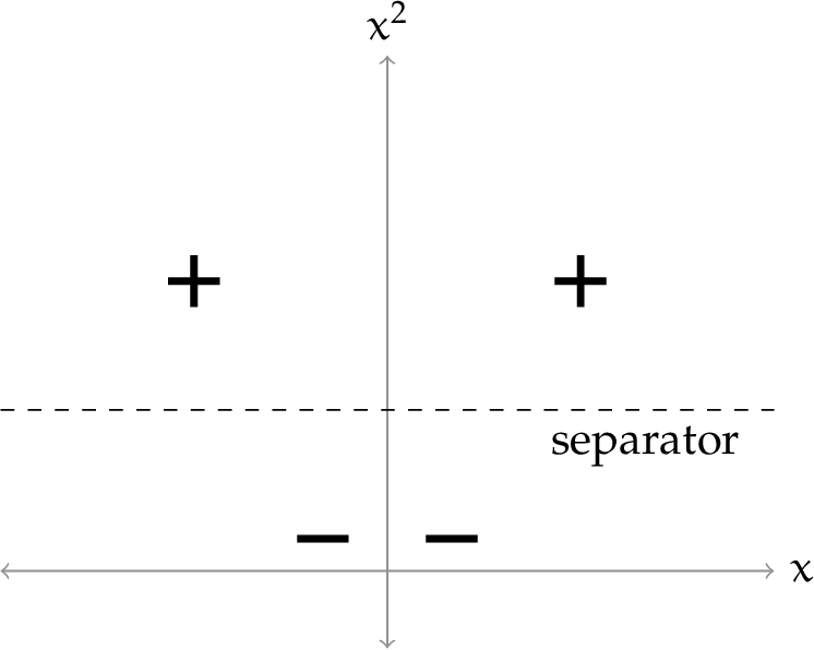
We can see that a linear separator in $\phi$ space is a non-linear separator in the original space. Let’s see more details:
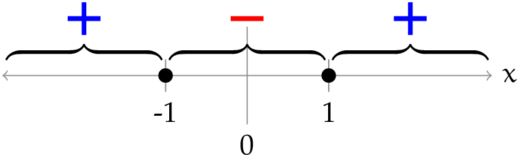
Consider the separator $x^2 - 1 = 0$, which labels the half-plane $x^2 - 1 = 0$ as positive. What separator does it correspond to in the original 1-D space? We have to ask the question: which $x$ values have the property that $x^2 - 1 = 0$. The answer is $+1$ and $-1$, so these two points constitute our separator, back in the original space. And we can use the same reasoning to find the region of 1D space that is labeled positive by this separator.
Polynomial basis
One technique used to solve non-linear problems is to transform a non-linear feature space into a linear one using a polynomial basis transformation. Specifically, this involves expanding the feature space by generating all combinations of input variables, up to a specified order $k$. This transformation allows linear classification algorithms, such as Perceptron, to be applied effectively in a higher-dimensional space where the data may become linearly separable.
Here is a table illustrating the $k$th order polynomial basis for different values of $k$:
| Order | $d = 1$ | In general |
|---|---|---|
| 0 | $[1]$ | $[1]$ |
| 1 | $[1, x]$ | $[1, x_1, \ldots, x_d]$ |
| 2 | $[1, x, x^2]$ | $[1, x_1, \ldots, x_d, x_1^2, x_1x_2, \ldots]$ |
| 3 | $[1, x, x^2, x^3]$ | $[1, x_1, \ldots, x_d, x_1^2, x_1x_2, \ldots, x_1x_2x_3, \ldots]$ |
Looking at the example table, we can see that we’ve added combinations of input variable like $x_1^2$, $x_1x_2$, …
So, what if we try to solve the xor problem using a polynomial basis as the feature transformation? We can just take our two-dimensional data and transform it into a higher-dimensional data set, by applying $\phi$.
Now, we have a classification problem as usual, and we can use the perceptron algorithm to solve it.
Let’s try it for $k=2$ on our xor problem. The feature transformation is:
$\phi((x_1, x_2)) = (1, x_1, x_2, x_1^2, x_1x_2, x_2^2)$
Study Question: If we use perceptron to train a classifier after performing this feature transformation, would we lose any expressive power if we let $\theta_0 = 0$ (trained without offset instead of with offset)?
My answer: Without offset, we would lose expressive power by setting $\theta_0 = 0$ in the perceptron model after the polynomial feature transformation.
Looking at the formular: $\phi((x_1, x_2)) = (1, x_1, x_2, x_1^2, x_1x_2, x_2^2)$. The number 1 at the beginning corresponds to the bias term, and it enables the perceptron algorithm to make non-zero intercept decisions, that means the decision boundary doesn’t have to go through the origin in the transformed feature space.
Setting $\theta_0 = 0$ means removing the bias term, which restricts the decision boundary to always pass through the origin of the feature space. This restriction will limit the range of the classification ability.
Back to the xor problem, after 4 iterations, perceptron algorithm finds a separator with coefficients $\theta = (0, 0, 0, 0, 4, 0)$ and $\theta_0 = 0$. This corresponds to:
\[0 + 0x_1 + 0x_2 + 0x_1^2 + 4x_1x_2 + 0x_2^2 + 0 = 0\]Then, the classification depends on the sign of $4x_1x_2$. That’s correct when looking back to the xor problem, when $x_1$ and $x_2$ are opposite on sign, the label will be $0$:
\[h(x) = sign(4x_1x_2)\]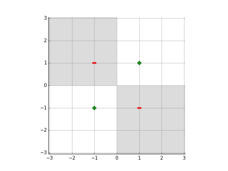
In the original 2-D space, the new space $\phi$ creates a curve plane (non-linear), but in the new 6-D space, it is a linear plane.
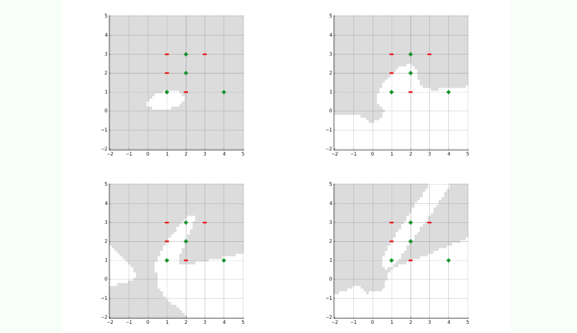
Here is a harder data set. After 200 iterations, we could not separate it with a second or third-order basis representation. Shown below are the results after 200 iterations for bases of order 2, 3, 4, and 5.
Hand-constructing features for real domains
In many machine-learning applications, we are given descriptions of the inputs with many different types of attributes, including numbers, words, and discrete features. An important factor in the success of an ML application is the way that the features are chosen to be encoded by the human who is framing the learning problem.
Discrete features
Encoding discrete features well is crucial because it helps machine learning models discover meaningful patterns. While some models can handle discrete inputs directly, the ones we study assume that input vector $x \in \mathbb{R}^d$, so we need smart ways to convert discrete values into numerical vectors.
Discrete values like color = red/green/blue, sexuality = male/female or day = Monday/Tuesday/… do not have inherent numeric meaning, but ML models work well on numeric features.
If we feed discrete values to numeric format - typically using strategies, so the models can process and learn more from them.
We’ll start by listing some encoding strategies, and then work through some examples. Let’s assume we have some feature in our raw data that can take on one of $k$ discrete values.
Numeric: Assign each of these values a number, like $1.0/k, 2.0/k, \dots, 1.0$. We might want to then do some further processing. This strategy is only meaningful when the discrete values really do signify some sort of numeric quantity. For example, sizes of shirt like S < M < L < XL can be transformed into $[0.25, 0.5, 0.75, 1.0]$. On the other hand, colors like red, green, blue do not have numerical meaning, so we can’t assign numbers like $1, 2, 3$.
Thermometer code: If the discrete values have a natural ordering, from $1, \dots, k$, but not a natural mapping into real numbers, a good strategy is to use a thermometer code. The basic concept is to transform a discrete value into a binary vector, in which the first values are $1$ and the rest are $0$. A basic example is, imagine that we have a satisfication attribute, from $1$ star to $5$ stars, we transform it into:
Factored code: If a value can be broken into parts (like car make and model), split and encode them separately. For example, we have a set of discrete values:
["Toyota Camry", "Toyota Corolla", "Honda Civic", "Honda Accord"]. We factor it into:$-$ Brand name:
["Toyota", "Honda"]$\$ $-$ Type of product:["Camry", "Corolla", "Civic", "Accord"]$\rightarrow$ Encoding:
Car Make (One-hot) Model (One-hot) Full Vector Toyota Camry [1, 0] [1, 0, 0, 0] [1, 0, 1, 0, 0, 0] Honda Civic [0, 1] [0, 0, 1, 0] [0, 1, 0, 0, 1, 0] One-hot encoding: Use when there’s no natural order. Each value becomes a binary vector with a single 1 in the position for that value. For example, there are 4 discrete values: $[“red”, “blue”, “green”, “yellow”]$. One-hot encoding generates 4 dimensions:
As an example, imagine that we have to encode blood types, which are drawn from the set ${A+, A-, B+, B-, AB+, AB-, O+, O-}$. There is no obvious linear numeric scaling or even ordering to this set. But there is a reasonable factoring, into two features: ${A, B, AB, O}$ and ${+1, -1}$. And, in fact, we can reasonably factor the first group into ${A, \text{not} A}$, ${B, \text{not}B}$, which we can treat $AB$ as having neither feature A nor feature B. So, here are two ways to encoding the whole set:
Using a 6-D vector, with four first dimensions to encode each of types of blood, the rest two dimensions are used to encode rhesus factor. For example:
$A+: [1, 0, 0, 0, 1, 0] \rightarrow$ the first
1is to indicate the type $A$, the rest1is to indicate the rhesus factor $-$.Using a 3-D vector, including:
Having $A$: $+1$; not $A$: $-1$ $\$ Having $B$: $+1$; not $B$: $-1$ $\$ Having $Rh+$: $+1$; having $Rh-$: $-1$
In this case, $AB+$ will be $(1.0, 1.0, 1.0)$ and $O-$ will be $(-1.0, -1.0, -1.0)$.
Text
The problem of taking a text (such a tweet or a product review) and encoding it as an input for a machine learning algorithm will be discussed much later in this course.
Numeric values
If a feature is already encoded as numeric value (heart rate, stock price, distance, …) then we should generally keep it as a numeric value.
There’re some exceptions that the numeric-based feature you’re analyzing has some “natural breakpoints”, like the age of 18 or 21, then it might make sense to divide into discrete bins and to use a one-hot encoding for some situations which we don’t expect a linear relationship between age and other features.
If you choose to leave a feature as numeric, it typically useful to scale it, so that it tends to be in the range $[-1, +1]$. The reason why we should perform this transformation is in the case you have one feature with much larger values than another, it will take the learning algorithm a lot of effort to find out the proper parameters.
So, we might perform the transformation: $\phi(x) = \frac{x - \bar{x}}{\sigma}$, where $\bar{x}$ is the average value of the $x^{(i)}$ and $\sigma$ is the standard deviation of the $x^{(i)}$. The resulting value will have mean $0$ and standard deviation $1$.
Then, of course, you might apply a higher-order polynomial-basis transformation to one or more groups of numeric features.
Study Question: Percy Eptron has a domain with 4 numeric input features, $(x_1, \dots, x_4)$ . He decides to use a representation of the form
\[\phi(x) = \text{PolyBasis}((x_1, x_2), 3) \mathbin{\hat{\ }} \text{PolyBasis}((x_3, x_4), 3)\]Solution: Percy Eptron applies a poly basis transformation of degree 3 to each two input features. So, in each group, the final feature input will be calcutated by the formular:
\[\binom{n + d}{d} = \binom{2 + 3}{3} = \binom{5}{3} = 10\]with $n$ is the initial number of input features, $d$ is the degree in the transformation.
So, two groups $(x_1, x_2)$ and $(x_3, x_4)$ have $20$ as the new number of features.
The choice to use transformation in each group is reasonable under the assumption that The features $x_1, x_2$ and $x_3, x_4$ interact strongly only in their own groups, and there is little or no meaningful interaction between the two groups.
In other words, we assume that nonlinear relationships exist primarily within each group.